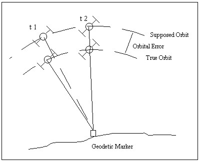
TIME-DEPENDENT CORRELATIONS USING THE GPS - A CONTRIBUTION TO DETERMINE THE UNCERTAINTY OF GPS-MEASUREMENTSDr. Volker SCHWIEGER, GermanyKey words: GPS, Synthetic Covariance Matrix, Time Series Analysis, Time-dependent Correlations, Uncertainty. 1. INTRODUCTIONA Geodesist always has to describe his results by adding a numerical value for the uncertainty of his observable to the observable itself. In general the standard-deviation or a confidence interval at a specified level of probability may be given. These stochastic values may be determined by empirical or synthetic methods. In both cases non-correlated measurements are generally assumed, mostly because knowledge about correlations is not available. The advantage of non-correlated measurements are more easy computation algorithms. This is a reason for the widespread acceptance of this simplification. For most of the classic geodetic measurement methods like e.g. levelling or angle measurement by a theodolite this holds partly true, but for the geodetic use of more complex measurement systems e.g. the Global Positioning System (GPS) correlations should not be neglected. These stochastic dependencies influence the estimation of the parameters like co-ordinates and especially of the respective uncertainties of these parameters. The geodetic use of the GPS for precise positioning relies on the positive correlations among simultaneous observations. The absolute positioning by GPS is uncertain to the approximately some meter level, because of different errors like the uncertainty of the GPS-satellite-orbits and path delays in the atmosphere acting on the GPS-signals. The measured ranges between a satellite and two neighbouring receiving antennas are falsified by almost the same errors leading to positive correlations among the observed ranges and the determined site co-ordinates. These correlations are well-known and software-packages take advantage of these correlations by using differences among the ranges or by modelling the correlations. Time-dependent correlations are well-known too. Most of the error sources influencing GPS-measurements variate only very slowly in time. Figure 2 demonstrates this fact for the orbit error. The slow time-dependent variation is documented in the literature (e.g. TEUNISSEN/KLEUSBERG 1998). This leads to differencing of successive observations to cancel the errors out. These time differences or the so called triple differences are used to detect cycle slips (e.g. HOFMANN-WELLENHOF 1994). Nevertheless they are often not taken into account for the determination of the empirical standard deviation of GPS determined co-ordinates. This is one reason for the over-optimistic estimation of the uncertainty of networks determined by GPS.
Figure 1: GPS orbit error as an example for time-dependent correlations One trend in research is the occurrence of correlations in time series for years as they are found at permanent active GPS-sites. If they are not taken into account, the uncertainty of the co-ordinates of the respective permanent GPS-site will be estimated too optimistic. Their knowledge will lead to correct uncertainty determination of observation related to active GPS-sites. The determination of these long-time time-dependent correlations may be done empirically respectively analytically or in a synthetic way. The following paper will give an insight into both estimation procedures. The influence of the determined correlations on the estimation of numerical values for the uncertainty - the standard deviations - will be outlined as well. 2. TIME-DEPENDENT CORRELATIONS USING THE GPS2.1 Synthetic Determination of Correlations for GPSFor synthetically determined variances and co-variances
respectively correlations a detailed image of all error sources and
the possible magnitudes has to be available. The influence of the
errors on the observations has to be known too. The theoretic
background for this type of uncertainty computation is called the
model of elementary errors, that has its roots in publications of the
last century (BESSEL 1837 and HAGEN 1837). PELZER (1985) expanded the
model including errors, that influence more than one observation
(functionally correlating errors). The multi-observation influence
gives the possibility to include correlations into the stochastic
model, the covariance matrix of the observations. Recently SCHWIEGER
(1999a) introduced another type of correlating error source, the
stochastically correlating errors. There the correlations among the
observations are due to correlated error sources like e.g. correlated
tropospheric fields. The Guide to the expression of uncertainty in
measurement (IOS 1995) calls this type of uncertainty determination a
type B estimation. With the exception of the type of elementary errors
introduced by SCHWIEGER (1999a), the Guide (GUM) deals with exactly
the same model. The general equation to determine the co-variance
matrix of the observations
Die first part of equation (1) contains the
influence of the not correlating elementary errors, the second part
describes the influence of the functionally correlating ones and the
last term stands for the stochastically correlating elementary errors.
The influencing matrices D, F and G contain
coefficients describing the influence of the errors, respectively the
variances and covariances, on the observations. Generally these
coefficients are the partial derivatives of a particular observation
with respect to a particular error. The matrices are diagonal (D and
G) or more or less completely filled (F). The covariance-matrices
describe the stochastic model of the error sources. In general they
are of diagonal nature ( Regarding most of the geodetic measurement techniques the knowledge about the influencing errors, that contribute to the uncertainty of the measurement is available (empirical determination or given by the manufacturer), with other words the covariance matrices of the different error sources and their influencing matrices may be written down and the resulting uncertainties including correlations may be determined according to equation (1). For some of the geodetic measurement techniques the determination of uncertainties is presented by different speakers within this workshop.
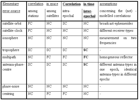
Table 1: Elementary errors of GPS monitoring
surveys ; One of the most complex measurement techniques are geodetic GPS-measurements. Up to now a complete model for determining uncertainties is not evaluated. SCHWIEGER (1999a) developed a model of elementary errors for GPS monitoring surveys valid up to maximum baseline lengths of 50 km. Table 1 gives a summary of the error sources that have to be taken into account and shows the occurrence of correlations in general. Special attention is given to time-dependent correlations covering years of observations, because the research was focussed on this topic. In any case the occurrence of time-dependant correlations is obvious for short periods as well as for periods covering years of observations.
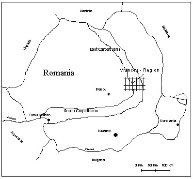
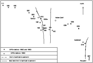
Figure 2: Location of the Vrancea network
Figure 3: Vrancea network
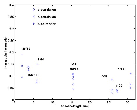
Figure 4: Interepochal correlations for selected baselines
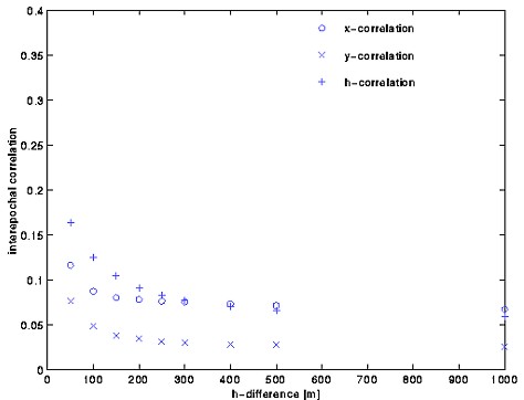
Figure 5: Interepochal height correlation in dependence of the height difference (baseline 36 -39) The research was realized for a vertical control network located in Romania in the Carpathian mountains (figures 2 and 3). It was observed by levelling in earlier times. In 1992 and 1993 the network was remeasured by GPS. So called interepochal correlations among the co-ordinates between the deformation epochs were determined by the synthetic methods described above. In Figure 4 the interepochal correlations determined for selected baselines of the network are shown. The computations result in maximum correlation coefficients of approximately 0.19. Simulations have shown that these correlations essentially depend on the baseline length, the height difference of the stations and the individual satellite configurations. The influence of the height difference for baseline 39-36 is presented in figure 5. The important influence of the day time and the season is documented by table 2 (chapter 3). The estimable correlations coefficients are of the magnitude that they have to be taken into account for the determination of uncertainties and other geodetic quality criteria (SCHWIEGER 1999a and 1999b). Some characteristic results are shown in chapter 3. The interepochal correlation coefficient reaches 0.38 for identical day time, season and satellite configuration. 2.2 Analytic Determination of Correlations
Figure 6: Original time series (Göttingen - Höxter, height component) The second possibility to determine time-dependent correlations is their analytic estimation. In this case the uncertainty as well as the correlations are estimated on the basis of empirical data. In IOS (1995) the procedure is called the estimation of a type A uncertainty. Because the paper deals with time-dependant correlations, we have to use the tools of time series analysis. The general procedure is trend separation, outlier elimination, and filtering. After these pre-processing steps are covariance-functions and FOURIER-transformed power-spectra are determined. The theory of time series analysis may be studied more in detail in the specialized literature (e.g BENDAT, PIERSOL 1971 or TAUBENHEIM 1969). For the determination of correlations for GPS time series two example data-sets were at the authors disposal. Five years of weekly solutions of the BKG (Bundesamt für Kartographie und Geodäsie) are used to investigate possible annual periods in the correlative behaviour. Fourteen days of hourly solutions of the LGN (Landesbetrieb Landesvermessung und Geo-Basisinformation Niedersachsen) shall give an insight into possible diurnal periods. The typical procedures are briefly summerized for the two time series. The trend elimination was realized using bit by bit linear regression analysis. The elimination of the outliers was done by linear interpolation and the filters were moving-average filters with different filter lengths ranging from 5 to 7. The results are presented in the form of autocovariance functions and power spectra for two exemplary data-sets. For more details regarding the procedure and the data-sets the author refers to JOHANNSEN (2000).
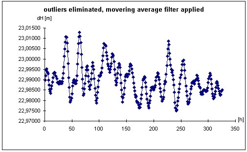
Figure 7: Time series after outlier elimination and applied moving average filter (Göttingen - Höxter, height component)
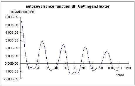
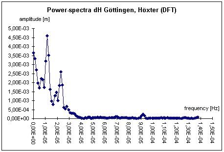
Figure 8: Autocovariance-function of the height-component (Göttingen-Höxter) Figures 6 to 9 illustrate the different data processing steps for the LGN-data. This data contains baselines with lengths up to 50 km located in the north of Germany (Lower Saxony). For presentation the height-difference between the cities of Göttingen and Höxter (baseline length: 48 km) is chosen. The analysis leads to a clearly visible diurnal period in the autocovariance function as well as a visible peak in the power-spectra. The correlation coefficient reaches a value of 0.52 for a period of one day and the peak of approximately 24 hours dominate the power-spectra. The exact value of the peak at 24.2 hours does not stand in contrast to the theoretical peak of 24 hours, because the availability of 1-hour-solutions restricts the uncertainty of the peak determination. The peak at the 12.1 hours, which occurs exactly at the half period with respect to the dominating 24.2 hour peak, is caused by the filter process and not by a real physical phenomenon. The correlation coefficient reaches an amount greater than the one estimated by synthetic means in chapter 2.1, because we deal with empirical data of two weeks. The influence of error sources with e.g. an annual period are not taken into account.
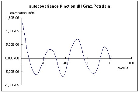
Figure 9: Power-spectra (Göttingen-Höxter, height-component) The BKG-data consists of baselines with lengths of continental dimensions; for presentation the height component of the 600-km-baseline Graz (Austria) - Potsdam (Germany) is chosen. The surprising result is a maximum peak at 27.3 weeks, and not at the expected 52 weeks. The peak stands for a semi-annual period, because the uncertainty of the peak again includes the theoretical semi-annual value of 26. In any case the result is a surprising one due to the expectation of an annual period. The annual period was expected because of e.g. tropospheric mismodelling. The cause for this rather unexpected correlative behaviour is supposed to be the ionosphere. In general some of the ionospheric layers show a semi-annual periodic behaviour (e.g. BAILEY et.al. 2000 and FEICHTINGER et.al. 1997). For modelling purpose (see chapter 2.1) the influence of the ionosphere was set to zero. This had its reason within the baseline lengths of maximum 50 km. WANNINGER (1994) points out that the ionospheric influence may arise up to approximately 0.2 ppm for the second order terms that remain after the GPS-2-frequency correction. For a 600 km baseline this influence has to be taken into account. Other possible semi-diurnal periods are the movement of the geo-centre (MONTAG 1997) or influences of the orbit determination, that should in general be eliminated by the orbit determination technique (TEUNISSEN, KLEUSBERG 1998).
Figure 10: Autocovariance-function (Graz - Potsdam, height-component)
Figure 11: Power-spectra (Graz - Potsdam, height-component) Additionally the attention has to be focussed on two aspects of the analysis. First it has to be stated that the power-spectra is much more suited to identify the semi-annual period. The autocovariance function shows the same period, but because of the higher correlation coefficient for one year, it could still be possible, that the two periods are of the same magnitude. Only the power-spectra shows, that this is obviously not the case. The magnitude of the correlations has to be regarded as the second aspect. It reaches up to 0.54 after one year. This value is much higher than it was modelled in chapter 2.1 by synthetic means. The reason may be given by the different error sources because of the extended baseline lengths in comparison to the example network in 2.1. In any case the correlations have to be taken into account for the determination of the uncertainty of GPS-determined co-ordinates (see chapter 3). 3. THE INFLUENCE OF CORRELATIONS ON GPS-UNCERTAINTYObviously correlations in hand influence the estimation of the parameters like co-ordinates as well as the respective standard deviation, because the stochastic model of the observations is different referring to a model neglecting these stochastic dependencies. It shall be stated that the comments of this chapter do not depend on the type of evaluation of uncertainty. To illustrate the influence of the correlations two
typical geodetic examples shall be given in the following. The most
used computational algorithm in Geodesy is the calculation of a mean.
If n not correlated values
If correlations among the values
with This equation is developed for the analysis of time series, but is valid for any correlations among observations. Another important computational algorithm is the
sum of observations. If two not correlated values
If correlations between the two values
Equations (3) and (5) both demonstrate the fact, that positive correlations decrease and negative correlations increase the respective standard deviations. This holds true for means and sums. If differencing of observations is the evaluation task, equation (4) is valid in the case of not correlated measurements. For the correlative case form (5) has to be transferred into
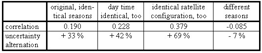
The equation demonstrates, that negative correlations decease and positive correlations increase the uncertainty of differences. Typical GPS-applications are the single, double and triple differences algorithms of GPS evaluation software. As another example the analysis of deformations may serve. In this case differences among co-ordinates of two or even more deformations epochs have to be realized. Table 2 shows interepochal correlations as well as alternations of the uncertainties of height-deformations, both estimated in a synthetic way (SCHWIEGER 1999a). The influence of day time, season and satellite configuration is obvious (compare chapter 2.1). The gain for the standard deviation of the height deformation (baseline 36-39) reaches an amount of almost 70 %, if identical satellite configurations, season and day time are simulated.
Table 2: Interepochal correlation coefficients and uncertainty alternation for different simulated conditions (baseline 36 - 39, height component) Summarising it can be said, that positive correlations are helpful in the case of differences among the observed quantities and negative correlations help, if a sum or a mean is estimated. In any case the correlations have to be taken into account to get a realistic image of the uncertainty values. 4. CONCLUSIONSCorrelations among GPS-observations as well as among GPS-determined co-ordinates may be determined in a synthetic way or in an empirical respectively analytic way. If the specifications of the GUM are used, it is referred to type A (empirical) and type B (synthetic) uncertainties that are quantified by standard deviations. For the synthetic determination the extended model of elementary errors is proposed. For the empirical estimation the well-known tools of time series analysis are used. The results are similar but not identical. Some differences especially regarding the periods of correlative elements have to be investigated. Nevertheless both methods seem to be appropriate for the determination of correlations and subsequently of uncertainties too. Independent of the way of estimation the time-dependant correlations have a magnitude that make it impossible to neglect these stochastic quantities. The uncertainties increase or decrease by a significant in some cases even high amount, if the correlations are correctly introduced into the evaluation process. ACKNOWLEDGEMENTAt this place the author thanks Ms Johannsen, who did the most work regarding chapter 2.2 within her diploma thesis. The colleagues of the LGN in Hannover were also very helpful, because they provide the data of their time series and compute the hourly solution for the scope of this research. At last I want to thank the colleagues of BKG, that helped, if questions concerning the weekly solutions arose. REFERENCESBAILEY, G.J., SU, Y.Z., OYAMA, K.-I., 2000, Yearly variations in the low-attitude topside ionosphere, Annales Geophysicae 18, pp 789-798, Springer. BENDAT, J.S., PIERSOL, A.G., 1971, Random Data: analysis and measurement procedures, New York/London/Sydney/Toronto, Wiley-Interscience. BESSEL, F.W., 1837, Untersuchungen über die Wahrscheinlichkeit von Beobachtungsfehlern, Astronomische Nachrichten, Vol. 15, p. 369ff. FEICHTNER, E., LEITINGER, R., 1997, A 22-year cycle in the F layer ionization of the ionosphere, Annales Geophysicae 15, pp 1015-1027, Springer. HAGEN, G., 1837, Grundzüge der Wahrscheinlichkeitsrechnung, Berlin. HOFMANN-WELLENHOF, B., LICHTENEGGER, H., COLLINS, J., 1994, GPS - Theory and practise, Wien/New York, Springer. IOS, 1995, Guide to the expression of uncertainty in measurement (GUM), International Organisation of Standardization (IOS), Switzerland. JOHANNSEN, K., 2000, Zeitreihenanalyse kontinuierlicher GPS-Messungen, diploma thesis (unpublished), Geodetic Institute, University of Hannover. MONTAG, H., 1997, Zu einigen Grundlagen globaler und regionaler Referenzsysteme, in: GPS-Anwendungen und Ergebnisse 1996, DVW-Schriftenreihe Nr. 28, Stuttgart, Konrad Wittwer. PELZER, H., 1985, Grundlagen der mathematischen Statistik und der Ausgleichungsrechnung, in: PELZER, H. (Ed.): Geodätische Netze in der Landes- und Ingenieurvermessung, pp 3-120, Stuttgart, Konrad Wittwer. SCHWIEGER, V., 1999a, Ein Elementarfehlermodell für GPS-Überwachungs-messungen - Konstruktion und Bedeutung interepochaler Korrelationen, Wissenschaftliche Arbeiten der Fachrichtung Vermessungswesen der Universität Hannover, Nr. 231. SCHWIEGER, V., 1999b, The effect of interepochal correlations in the analysis of monitoring surveys, Proceedings on 9th International FIG Symposium on deformations measurements, pp 234-244, Olsztyn. SEEBER, G., 1993, Satellite Geodesy: foundations, methods and applications, Walter de Gruyter, Berlin/New York. TAUBENHEIM, J., 1969, Statistische Auswertung geophysikalischer und meteorologischer Daten, Leipzig, Akademische Verlagsgesellschaft Geest & Portig. TEUNISSEN, P.J.G., KLEUSBERG, A., 1998, GPS for Geodesy, Berlin/Heidelberg/New York, Springer. WANNINGER, L., 1994, Der Einfluß der Ionosphäre auf die Positionierung mit GPS, Wissenschaftliche Arbeiten der Fachrichtung Vermessungswesen der Universität Hannover, Nr. 201. BIOGRAPHICAL NOTEDr. Volker Schwieger
Scientific Interests
CONTACTDr. Volker Schwieger 22 April 2001 This page is maintained by the FIG Office. Last revised on 15-03-16. |


 with
with